INSTANTANEOUS WATER HAMMER EQUATION
The water hammer instantaneous valve closure calculation predicts the maximum increase in pressure that will occur due to a sudden valve closure.
Each series of articles are written by pipe flow analysis engineers from Datacor's Pipe Flow Modeling Division. As industry leaders in water hammer and surge analysis, Datacor Pipe Flow Modeling has collected models and data from projects around the world to use as reference materials for published technical papers, case studies, and blogs. Visit Datacor.com/products/impulse for more information on analysis tools.
Water Hammer Concepts:
Instantaneous Water Hammer Equation
The instantaneous water hammer equation, often referred to as the Joukowsky Equation, can be used to predict the maximum head/pressure rise that will occur in a piping network due to an instantaneous velocity change. The severity of the pressure change is determined by the change in momentum, the wave speed in the fluid, and the density of the fluid at the origin of the flow disturbance.
The instantaneous water hammer equation is defined as: ΔP = -ρaΔV
Where
ΔP= pressure rise at the location of the velocity change
ρ = fluid density
a = wave speed
ΔV = change in velocity
How was the Instantaneous Waterhammer Equation derived?
The instantaneous water hammer equation is derived from the equations for conservation of mass and momentum as follows.
Consider a one-dimensional fluid flow shown in Figure 1 where the local velocity has been disturbed a small amount (ΔV). This disturbance can be caused by a progressing valve closure for example. This small disturbance to flow causes a wave of small disturbances in pressure (ΔP) and density (Δρ) as the fluid’s kinetic energy is converted to potential energy. This wave travels away from the original disturbance at the wave speed, a. This scenario is represented in the below control volume upstream of the flow disturbance.

Figure 1: Control Volume over which a mass and momentum balance will be performed.
The conservation of mass principle can be applied to the above control volume as follows, where A is the cross-sectional area:

From Equation 2 the flux term can be expanded and the time derivative can be simplified, resulting in the following Equation 3:

The density is only changing in the volume swept by the wavefront (moving at speed a, against the fluid velocity) over the time step. Therefore, only the change in density within this control volume must be considered, as the other terms would cancel out. The volume swept by the wave is:
![]()
Substituting the swept volume equation into Equation 3 results in the following Equation 5:![]()
Further simplifying Equation 5 by dividing through by cross-sectional area, A, results in the following simplified equation for conservation of mass over the control volume:
![]()
The conservation of momentum of the control volume can be expressed as follows:
![]()
The sum of forces over the control volume will include all hydraulic forces. Assuming that the pipe is frictionless, the hydraulic forces can be calculated by the change in pressure over the area as follows:
![]()
The right-hand side of Equation 7 can be expanded into a time derivative and flux term:
Equation 4 for swept volume can be applied to simplify the time derivative in Equation 9 as follows: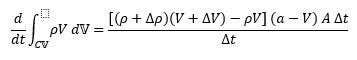
The flux term in Equation 9 can be simplified as follows![]()
Combining and simplifying the above equations into Equation 7 results in the below equation for pressure drop:![]()
Equations 6 and 12 from the conservation of mass and conservation of momentum equations can be combined and simplified, resulting in Equation 1 given above.
What are the physical implications of the Instantaneous Water Hammer equation?
The instantaneous water hammer equation is most often used to predict the pressure rise that will occur at the point where flow is halted in the system. In a frictionless system, this pressure rise would be transmitted following the Waterhammer Cycle through the pipes in the system. In an actual system, this maximum pressure rise will be reduced by frictional losses as the pressure wave traverses the system.
Often, the Joukowsky calculated pressure rise will accurately predict the maximum possible pressure rise caused by a valve closure. However, there are several cases where the Joukowsky equation does not adequately predict the maximum pressure rise. These scenarios are discussed further in the article When the Joukowsky Equation Fails.
The variables in the Instantaneous Waterhammer equation can be used to conceptually inform system design. Fluids with lower density will experience a lower pressure rise following an instantaneous valve closure due to their lower momentum. Similarly, a slower flow will have less potential for significant pressure rise during an instantaneous valve closure. A pipe with a low modulus of elasticity or small thickness will allow for a lower wave speed in the pipes, and thus a lower possible pressure rise.
The instantaneous water hammer equation can also be used to predict the pressure drop that will occur due to an instantaneous increase in flow, such as due to a fast valve opening. The same conceptual design concepts described above can be applied by simply replacing pressure rise with magnitude of pressure drop.
Reducing Pressure Rise – A Numerical Example
Consider the simple model below in Figure 2 with a valve that will be closed instantaneously. The system fluid is Water at 72°F (21°C), and the pipes are Steel-ANSI Schedule 40. The inputs and resulting pressure rise are detailed in Table 1 below.
Table 1: Relevant input and output parameters for valve closure example shown in Figure 2.
| Parameter | Value |
| Fluid Density | 62.3 lbm/ft3 (1000 kg/m3) |
| Wave speed | 3960 ft/s (1210 m/s) |
| Initial velocity | 2.06 ft/s (0.628 m/s) |
| Resulting Pressure Rise | 110 psi (7.6 bar) |

Figure 2: Example Model built in AFT Impulse. The valve is modeled to close linearly over 0.5 seconds.
Consider the components of the Joukowsky equation and the theoretical options discussed above to reduce this pressure rise.
The first option to reduce pressure rise is lowering the fluid density. Note that the fluid properties including density will also impact the wave speed, so this correlation is not direct. Changing the system temperature is one possibility to change the density of the fluid; however, even with large changes in temperature the change in fluid density will typically be minimal. Choosing a different system fluid to vary the density will provide a more interesting discussion. For example, ethanol at the same temperature will have a density of 49.2 lbm/ft3 (789 kg/m3), about 20% less than the density of water. The wave speed in ethanol will be 5020 ft/s (1530 m/s), about 25% larger than the wave speed in water. If the initial velocity is equivalent to the original case, the pressure rise using ethanol in the pipe will be the same as the pressure rise using water. The inputs and resulting pressure rise are summarized in Table 2. In this case, it was a coincidence that the pressure rise remained the same., but it is often the case that changing the density will have a minimal impact on the pressure rise.
Table 2: Relevant input and output parameters for valve closure example with decreased density.
| Parameter | Value |
| Fluid Density | 49.2 lbm/ft3 (789 kg/m3) |
| Wave speed | 5020 ft/s (1530 m/s) |
| Initial velocity | 2.06 ft/s (0.628 m/s) |
| Resulting Pressure Rise | 110 psi (7.6 bar) |
Next consider using a material with a lower modulus of elasticity, such as PVC. Using water at 72˚F, the wave speed in PVC will be about 1418 ft/s (432 m/s), about 64% less than the wave speed in Steel-ANSI. Assuming the initial velocity remains equivalent, then a direct correlation exists between wave speed and pressure rise. Thus, the pressure rise is reduced to about 40 psi (2.8 bar) at the valve, which is about 64% of the initial pressure rise. Table 3 below summarizes the adjusted inputs and pressure rise.
Table 3: Relevant input and output parameters for valve closure example with decreased wave speed due to change in pipe material.
| Parameter | Value |
| Fluid Density | 62.3 lbm/ft3 (1000 kg/m3) |
| Wave speed | 1418 ft/s (432 m/s) |
| Initial velocity | 2.06 ft/s (0.628 m/s) |
| Resulting Pressure Rise | 40 psi (2.8 bar) |
Finally, consider decreasing the initial velocity. For a constant pipe diameter, a decrease in velocity is directly proportional to the change in the pressure rise at the valve. However, if the velocity is decreased by increasing the pipe diameter, then the wave speed will also be affected, meaning that the change in velocity will no longer be directly proportional to the change in pressure rise. Thus, if the flow rate is directly decreased by 25%, such as through a flow metering device, then the pressure rise will also decrease by 25%, which would result in an 82 psi pressure rise as is shown in Table 4. If instead the pipe diameter is increased to decrease the velocity by 25%, the pressure rise would be about 80 psi. This minor difference is due to the fact that changing the pipe diameter will also change the wave speed in the pipe.
Table 4: Relevant input and output parameters for valve closure example with decreased initial velocity.
| Parameter | Value |
| Fluid Density | 49.2 lbm/ft3 (789 kg/m3) |
| Wave speed | 3960 ft/s (1210 m/s) |
| Initial velocity | 1.55 ft/s (0.472 m/s) |
| Resulting Pressure Rise | 82 psi (5.6 bar) |
In an actual system, many of the variables discussed above cannot be isolated as was assumed for this example. However, understanding the instantaneous water hammer equation and its parameters is still invaluable to evaluating and preventing potential pressure surge.